Interpolation and Density Estimation

Author

Yannic Celio

Interpolation and Density Estimation

This document contains the solutions for interpolation (NO₂) and density estimation (red kite data).

#Setup

# Packages
library(sf)
library(dplyr)
library(ggplot2)
library(gstat)
library(terra)
library(spatstat.geom)
library(spatstat.explore)

sf_use_s2(FALSE)

# Data
data_path <- "C:/Users/celio/Inter Dens/Data"

luft <- st_read(file.path(data_path, "luftqualitaet.gpkg"), layer = "luftqualitaet", quiet = TRUE)
schweiz <- st_read(file.path(data_path, "schweiz.gpkg"), layer = "schweiz", quiet = TRUE)
milan <- st_read(file.path(data_path, "rotmilan.gpkg"), layer = "rotmilan", quiet = TRUE)

luft <- st_transform(luft, 2056)
schweiz <- st_transform(schweiz, 2056)
milan <- st_transform(milan, 2056)

Interpolation Exercise 1: IDW

grid <- st_make_grid(schweiz, cellsize = 10000, what = "centers") |>
  st_sf() |>
  st_intersection(schweiz)

idw_res <- gstat::idw(
  value ~ 1,
  luft,
  newdata = grid,
  idp = 2,
  nmin = 4,
  nmax = 14
)

[inverse distance weighted interpolation]

ggplot() +
  geom_sf(data = idw_res, aes(color = var1.pred), size = 1.5) +
  geom_sf(data = schweiz, fill = NA, color = "black") +
  geom_sf(data = luft, color = "red", size = 1) +
  scale_color_viridis_c(name = expression(NO[2])) +
  labs(title = "IDW interpolation of NO2") +
  theme_minimal()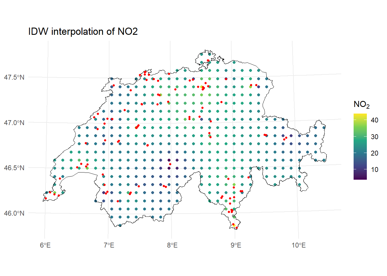

# IDW → raster
idw_vect <- vect(idw_res)
idw_r <- rast(ext(idw_vect), resolution = 10000, crs = st_crs(schweiz)$wkt)
idw_r <- rasterize(idw_vect, idw_r, field = "var1.pred")

plot(idw_r, main = "IDW interpolation raster")
plot(vect(schweiz), add = TRUE)
points(st_coordinates(luft), pch = 16, cex = 0.5)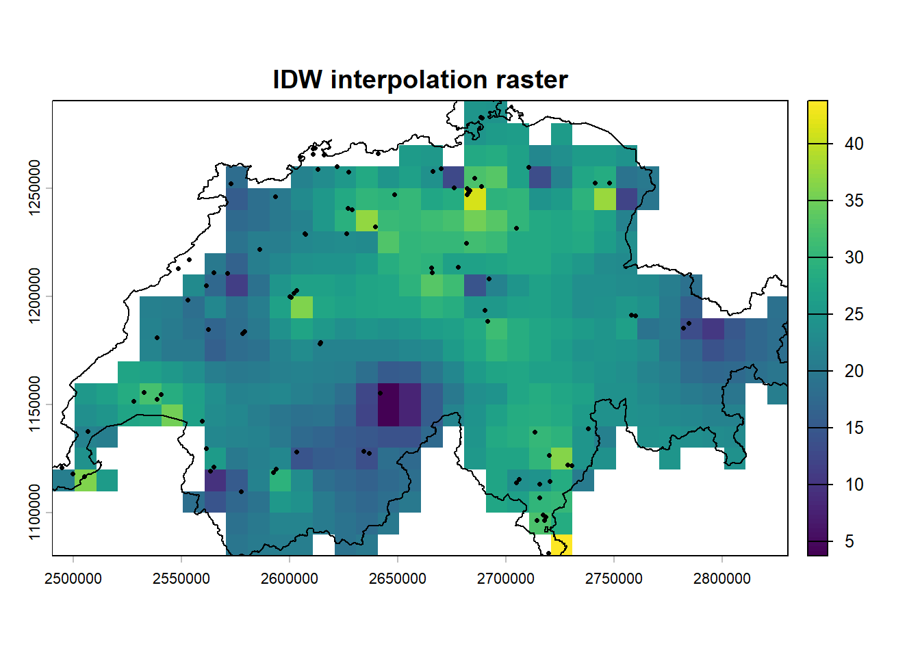

Interpolation Exercise 2: Nearest Neighbour

vor <- st_voronoi(st_union(luft)) |>
  st_collection_extract("POLYGON") |>
  st_as_sf()

vor <- st_join(vor, luft) |>
  st_intersection(schweiz)

ggplot() +
  geom_sf(data = vor, aes(fill = value), color = NA) +
  geom_sf(data = schweiz, fill = NA, color = "black") +
  geom_sf(data = luft, color = "red", size = 1) +
  scale_fill_viridis_c(name = expression(NO[2])) +
  labs(title = "Nearest neighbour (Voronoi)") +
  theme_minimal()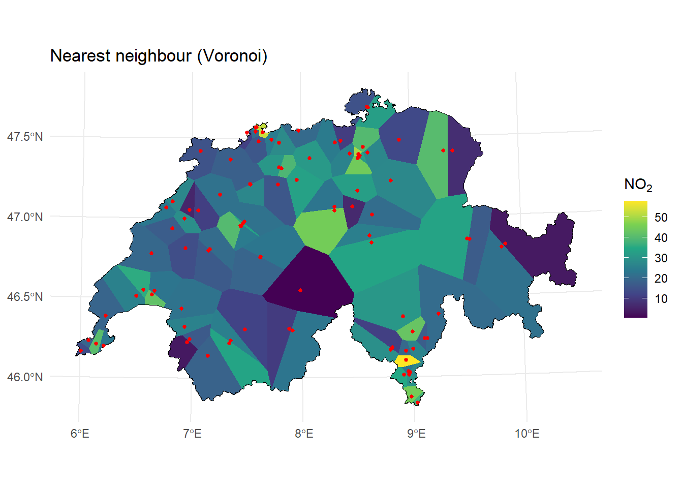

Density Estimation Exercise 1: Kernel Density Estimation

pp <- as.ppp(st_geometry(milan))

bw.diggle(pp)

   sigma 
25.16005

bw.CvL(pp)

   sigma 
38038.72

bw.scott(pp)

 sigma.x  sigma.y 
4302.234 1829.652

bw.ppl(pp)

  sigma 
944.463

sigma <- c(5000, 5000)

kde <- density(pp, sigma = sigma, eps = 500)
kde_r <- rast(kde)

plot(kde_r, main = "Kernel density estimation")
points(pp, col = "grey", pch = 16, cex = 0.2)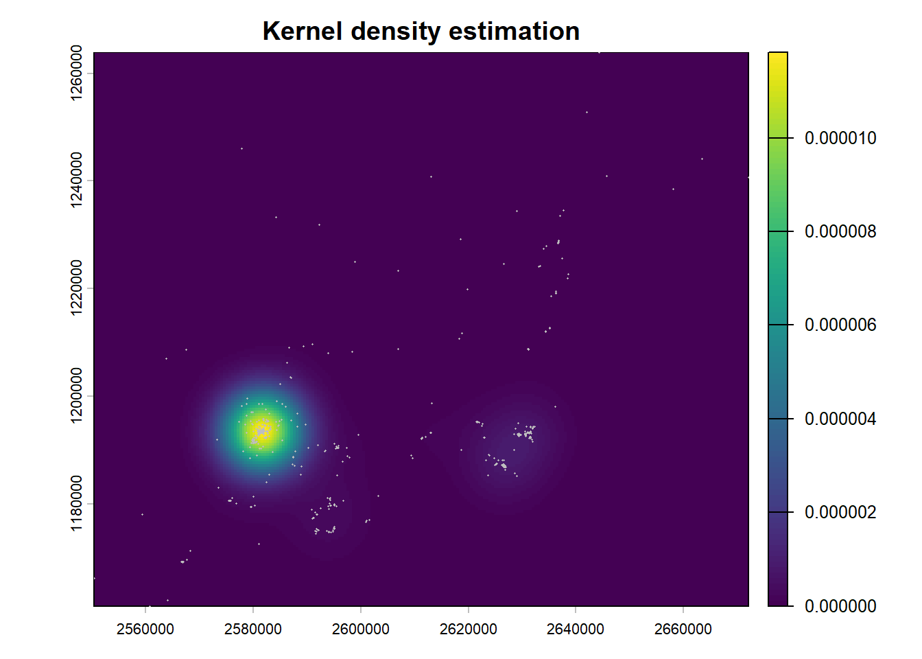

Density Estimation Exercise 2: Voronoi

# =========================
# VORONOI (POINT STRUCTURE)
# =========================
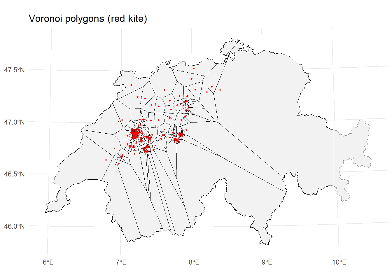
vor_m <- st_voronoi(st_union(milan)) |>
  st_collection_extract("POLYGON") |>
  st_sf()

vor_m <- st_intersection(vor_m, schweiz)

ggplot() +
  geom_sf(data = schweiz, fill = "grey95", color = "grey60") +
  geom_sf(data = vor_m, fill = NA, color = "black", linewidth = 0.2) +
  geom_sf(data = milan, color = "red", size = 0.5) +
  labs(title = "Voronoi polygons (red kite)") +
  theme_minimal()